Adjusting SOLPS-ITER input
You have created a SOLPS simulation, run it until it converged and learned accessing and plotting its results. Now it's time to coax it into giving you the results you want. In interpretative modelling, you have experimental diagnostic measurements you wish to match. In predictive modelling, you have scalings, core code predictions and similar plasmas in other tokamaks. To match the desired results as closely as possible, you need to adjust your SOLPS-ITER simulation by tweaking its input parameters, run it until converged again, tweak its inputs, run, rinse and repeat.
This tutorial covers:
- What are SOLPS-ITER inputs?
- Boundary conditions 101
- Four principle SOLPS-ITER inputs
- Other input parameters of note: heat flux limiters, divertor target grounding, and sheath heat transmission coefficients
- Expected fidelity
Once you have mastered these, you can move on to features described in the Feature blog:
- Overfitting diffusion coefficients
- Implementing drifts
- Playing with gas puffing and pumping
- Adding impurities
- Switching to wide grids
Input parameter overview
To look up information on boundary conditions and SOLPS-ITER input parameters, use our B2.5 switch database. It has colours and a search function.
What are SOLPS-ITER inputs?
In general, a SOLPS-ITER "input" is any information you feed to SOLPS-ITER. The magnetic equilibrium is one such input, or the wall outline, or the fact that recycled plasma particles recycle as deuterium molecules D2. Within this tutorial, however, SOLPS inputs are numbers you change in the text input files as you run a SOLPS-ITER simulation. Eventually, you'll become familiar a lot of input files, but for now you only need to worry about three: b2.boundary.parameters, b2.transport.parameters and b2mn.dat.
The simplest way to change a SOLPS input is to open the corresponding text file, find the position where the parameter is given and change the parameter value.
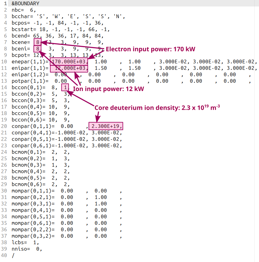
Example boundary condition file b2.boundary.parameters with marked locations of boundary condition type (BCCON, BCENE, BCENI) and value (CONPAR, ENEPAR, ENIPAR).
There have been efforts to automatise this through a more user-friendly interface, such as the SOLPS-inputsopen_in_new Python package written by Jan Hečko. A great progress has been made in converting the EIRENE master input file input.dat into the JSON format eirene.input.json, where a superfluous white space (such as one newline too many at the end of the file) will no longer crash your SOLPS. To start with, however, it is useful to learn working with the text files, even if they seem completely incomprehensible at first.
Most SOLPS inputs fall into two categories:
-
Switches, found in
b2mn.datfor B2.5 (andinput.datfor EIRENE). They typically control behaviour of the code, such as "don't solve the potential equation" or "multiply the anomalous conductivity by a bajillion". If the simulation behaves, you will typically adjust them only to set the simulation runtime. -
Boundary conditions and transport parameters, found in
b2.boundary.parametersandb2.transport.parameters, respectively. These control the plasma parameters: plasma density, how much power enters the SOL, how the sheath works etc. While adjusting a simulation to get the result you want, you will spend most of your time editing these.
Boundary conditions 101
"I've opened
b2.boundary.parameters. It's just numbers and letters. How do I work with this?"
B2.5, the plasma solver of SOLPS-ITER, is a finite volumeopen_in_new solver of the Braginskii equationsopen_in_new. The Braginskii equations inform it about what's going on in the middle of its computational region, but it needs to be told what happens at its boundaries. For example, the Braginskii equations have no idea what's happening inside the electric sheath enveloping the divertor targets. Consequently, B2.5 has to be told that the sheath accelerates ions up to the sound speed (boundary condition for the momentum equation), eats up plasma energy via the sheath heat transmission coefficient (boundary condition for the electron and ion energy equations) and absorbs every plasma particle to release it as a recycled neutral (boundary condition for the continuity equation). Boundaries envelop the B2.5 computational domain from all sides, and in the structured SOLPS-ITER version (which this tutorial works with, as opposed to the Wide Grids SOLPS), the boundaries all have colloquial names: North, South, West and East.
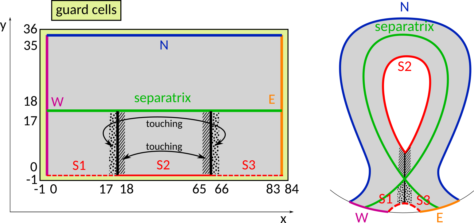
Study this scheme carefully. Keep it printed somewhere until you memorise it. It will come up often when working with structured grids.
B2.5 boundary naming conventions for other magnetic topologies
Different magnetic topologies (upper single null, double null) have different names for the B2.5 boundaries. Find them in the SOLPS manual.
The boundaries of the B2.5 computational region (in the lower single null configuration) are:
- South (S2, S1, S3): "Core boundary" (innermost flux surface) and two PFR boundaries. The core boundary controls the plasma density and input power, the PFR boundaries control the particle and power fluxes to the PFR wall.
- North (N): Far SOL boundary (outermost flux surface). Controls particle and power fluxes to the first wall.
- West (W): Inner target boundary. Controls the inner target sheath.
- East (E): Outer target boundary. Controls the outer target sheath.
It's important to know the colloquial names for B2.5 boundaries because they are used to index B2.5 boundary condition files. In the b2.boundary.parameters shown above, there are the lines:
 bcchar= 'S', 'W', 'E', 'S', 'S', 'N',
 bcpos= -1, -1, 84, -1, -1, 36,
 bcstart= 18, -1, -1, -1, 66, -1,
 bcend= 65, 36, 36, 17, 84, 84,
These lines mean that wherever boundary conditions are listed for all B2.5 boundaries, there will be 6 numbers and they will correspond, respectively, to boundaries S2 (core), W (outer target), E (inner target), S1 and S3 (PFR) and N (far SOL). You can tell the difference between the three South boundaries using the indices. Perusing the B2.5 switch documentationopen_in_new for the meaning of BCPOS, BCSTART and BCEND, you can learn that the S2 (core) boundary has the \(y\) (radial) index -1 and poloidally (in \(x\)) spans from cell 18 to 65, that is, from inner X-point to outer X-point.
Knowing the number of boundaries is useful for orientation in SOLPS input files. Wherever indices run from 1 to 6, you can be pretty sure they're listing the individual B2.5 boundaries in the order given by BCCHAR. Besides the 6 B2.5 boundaries, another recurring list that you'll encounter in the example b2.boundary.parameters file runs from 1 to 2. This is the list of all ion species. Its index is usually denoted is (Index of Species) and in this example file, it includes two "ion" species only: deuterium atom neutrals and deuterium (singly charged) ions. (Molecules are not covered by B2.5, only by EIRENE.) The boundary conditions of the continuity and momentum equation are given separately for every ion species. That's why you have:
 bcmom(0,1)=  2,  2,
 bcmom(0,2)=  1,  3,
 bcmom(0,3)=  1,  3,
 bcmom(0,4)=  2,  2,
 bcmom(0,5)=  2,  2,
 bcmom(0,6)=  2,  2,
 mompar(0,1,1)=  0.00    ,  0.00    ,
 mompar(0,2,1)=  0.00    ,  1.00    ,
 mompar(0,3,1)=  0.00    ,  1.00    ,
 mompar(0,4,1)=  0.00    ,  0.00    ,
 mompar(0,5,1)=  0.00    ,  0.00    ,
 mompar(0,6,1)=  0.00    ,  0.00    ,
 mompar(0,2,2)=  0.00    ,  0.00    ,
 mompar(0,3,2)=  0.00    ,  0.00    ,
BCMOM is given on 6 lines (corresponding to each of the 6 B2.5 boundaries) and each line has 2 values (corresponding to D0 and D+). Perusing the description of BCMOM = 2 in the B2.5 switch documentationopen_in_new, you will find this boundary condition only has one free parameter: MOMPAR(,,1). However, boundary condition BCMOM = 3 has two free parameters: MOMPAR(,,1) and MOMPAR(,,2). That is why there are 8 lines for MOMPAR: 6 of them list MOMPAR(,,1) and 2 of them list MOMPAR(,,2). Reading the indices in the brackets, you can find the exact place where you need to edit a number to change a SOLPS input.
There are many available boundary conditions
As of February 2026, there are 28 available boundary conditions for the ion energy equation BCENI in the "structured grids" SOLPS-ITER 3.0.9, and the list is growing. You can prescribe the sheath (BCENI=3), you can prescribe the sheath but different (BCENI=11,12), you can prescribe the sheath but compatible with drifts (BCENI=15)... At this point, as you read this introductory tutorial, don't worry about all of these options and stick to the default ones, which were pre-generated in the stencil files. But later, once you've mastered the basics and you move on to the Feature blog, you will study this list of boundary conditions and choose the best one for your simulation.
Four principle SOLPS-ITER inputs
The boundary condition (BC) files SOLPS has pre-generated for you contain a simple set of boundary conditions. When you first tweak a SOLPS simulation, you'll use the parameters of these boundary conditions. For example, the boundary condition for the core (South, S2) boundary of the deuterium ion continuity equation is BCCON = 1 ("fix a certain density at this boundary") and its parameter CONPAR is the density to be fixed.
There are four principle SOLPS simulation inputs which you will, one way or another, set in every simulation. These are the core main ion density \(n_{i,core}\), the input power \(P_{sep}\), the particle diffusion coefficient \(D_n\) and the electron and ion thermal diffusion coefficient \(\chi_{e,i}\).
The core density \(n_{i,core}\) is used with the continuity equation boundary condition BCCON = 1 ("prescribe the value of the density") at the core (S2) boundary, species index IS = 1 (deuterium ions). In b2.boundary.parameters, its value is on the line CONPAR(0,1,1). Put in the required density in part/m3. Increasing the core density will make the entire plasma density rise.
The input power \(P_{sep}\) is often called the power crossing the separatrix. This is not entirely accurate as the input power actually crosses the innermost flux surface of the SOLPS simulation region (the S2 boundary). The total input power has to be split between electrons and ions; it is usually split in half. It is used with the electron and ion energy boundary condition BCENE = BCENI = 8 ("prescribe the total electron/ion heat flux with constant flux density"). In b2.boundary.parameters, it is on the line ENEPAR(1,1) or ENIPAR(1,1). Put in half of total the power crossing the separatrix in W. Increasing the input power will make the plasma a little hotter and deposit more power on the divertor targets.
The particle diffusion coefficient \(D_n\) is used with the transport flag FLAG_DNA=1 ("transport model flag for electron/ion heat diffusivity - constant diffusivity"). In b2.transport.parameters, its value is given at PARM_DNA. Put in the required particle diffusion coefficient in m2s-1. Increasing \(D_n\) will flatten the density profile. Since the core density is fixed, this will make the density in the whole edge plasma rise.
The electron and ion thermal diffusion coefficient \(\chi_{e,i}\) is used with the transport flags FLAG_HCE=1 and FLAG_HCI=1 ("transport model flag for density-driven diffusion - constant diffusivity"). In b2.transport.parameters, its value is given at PARM_HCE and PARM_HCI. Put in the required thermal diffusion coefficient in m2s-1, usually the same for electrons and ions. Increasing \(\chi_{e,i}\) will flatten the respective temperature profile. Since the input power is fixed, this leaves the separatrix \(T_{e,i,sep}\) approximately the same, increases core temperatures and decreases SOL temperatures.
Why are these the principle SOLPS inputs?
Input power and plasma density (controlled by gas puff throughput) are two principle discharge controls in a real tokamak experiment. Diffusion coefficients cover an important deficiency at the heart of SOLPS: its inability to self-consistently describe radial transport. (If you thought SOLPS was much better at describing parallel transport, wait until you hear about heat flux limiters.) Together, these four parameters determine the separatrix density \(n_{e,sep}\) and temperature \(T_{e,sep}\), which are the strongest drivers of edge plasma transport.
Learn more about diffusion coefficients
While core density \(n_{i,core}\) and input power \(P_{sep}\) have straightforward values and effects, diffusion coefficients are more opaque, especially in predictive simulations. Read more about them in the feature blog entry Diffusion coefficients.
Other input parameters of note
Heat flux limiters
Electron and ion heat flux limiters \(\alpha_e\) and \(\alpha_i\) (attempt to) emulate kinetic effects in SOL parallel transport of heat. They are set in the b2.transport.parameters file, using the switches cflme and cflmi. The lower heat flux limiters are, the higher the corresponding parallel temperature gradient \(\nabla_\parallel T\). Under fixed input power \(P_{sep}\), lowering \(\alpha\) will make upstream \(T\) increase and target \(T\) decrease. The effect is much stronger for ions than for electrons.
How to set heat flux limiters [Kateřina's article in the making]:
- I don't care, just give me a value. Use \(\alpha_e = \alpha_i = 1.5\). [Fundamenski 2005open_in_new]
- I want to do this properly. Make a four-point parameter scan: \([\alpha_e, \alpha_i] = [1000, 1000], [1000, 0.1], [0.1, 1000], [0.1, 0.1]\). Assess the sensitivity; it will be higher for ions and it will depend on the SOL transport regime. If the simulation is not sensitive to \(\alpha\), it doesn't matter which value you choose. If it is sensitive, choose \(\alpha\) in conjunction with input power split \(P_{sep,i} / P_{sep,e}\) to achieve the desired upstream and target temperatures at the separatrix. In all, treat electron and ion heat flux limiters independently.
More reading
- W. Fundamenski, Parallel heat flux limits in the tokamak scrape-off layeropen_in_new, Plasma Physics and Controlled Fusion 47 (2005) - the best review of heat flux limiting to date
- Kateřina's PhD thesisdownload, chapter 5 Heat flux limiting
Divertor target grounding
Currents in the edge plasma can be significantly affected depending on whether the divertor target tiles are grounded or floating. Control the target biasing in the potential equation boundary condition, BCPOT = 3 (sheath) or BCPOT = 11 (sheath, but better), using the parameter POTPAR(,2).
Sheath heat transmission coefficients
The electron and ion sheath heat transmission coefficient \(\gamma_e\) and \(\gamma_i\) affect the amount of energy the divertor target sheath drains from the plasma. They can be partially controlled in the electron and ion energy equation boundary condition, BCENE/I = 3, 11, 12, 15 (all variants of the sheath), using the parameter ENE/IPAR(,1). Beware, the ENE/IPAR parameter has different meaning for each boundary condition number.
More reading
- Interpretative simulations of COMPASS, section Target parallel energy flux density
Expected fidelity
An important part of adjusting SOLPS-ITER simulations is knowing when to stop. You can tweak your simulation until it gives you exactly what you wanted, or you can stop at "good enough" and go for a walk in the woods.
What level of fidelity you can expect from SOLPS varies greatly between upstream and target. Upstream can be easily matched to within 20 % accuracy. The separatrix \(n_{e,sep}\) and \(T_{e,sep}\) directly respond to the core density \(n_{i,core}\) and input power \(P_{sep}\), while the shape of their profiles can be fine-tuned using diffusion coefficients. On the other hand, if you get the target plasma parameters within a factor of two, you've done a great job. Broadly speaking, if you match the qualitative measures of the SOL transport regime (pressure and power losses, parallel \(T_e\) gradient, plasma radiation patterns, peak target \(T_e\) and \(q_\parallel\)), you can pat yourself on the shoulder and say "my job here is done".
I always remember that one interpretative simulationopen_in_new of ASDEX Upgrade detachment where the outer target \(T_e\) was 10x lower and the inner target was qualitatively wrong, but which was called a success because if you multiplied target \(T_e\) and \(n_e\), the errors compensated and you got a reasonable profile of \(p_e\). On the outer target.
The bar is not that high.
Bayesian inference
A promising approach toward tweaking SOLPS-ITER input and gauging their uncertainties is Bayesian inference. At IPP Prague, it is currently being investigated by Jan Hečko (mail hecko@ipp.cas.cz) and Šimon Soldát. It promises to adjust SOLPS input parameters for you automatically and to give you uncertainties of these inputs. Stay tuned for Honza's article in the making!